About six or seven years ago I switched from using the QWERTY keyboard layout to the Dvorak layout. It was quite a big change as I had been using QWERTY for about 15 years. I thought it would be useful to describe the pros and cons, operating system support, and other things to consider for those who are thinking of making the switch.
Dvorak Keyboard Layout
Motivation
I had two motivations to consider switching away from QWERTY. The first was the prospect of being able to type faster and with less risk of repetitive strain injury by using a more efficient layout. Pain in my fingers and joints was rare, only ocurring after programming for several hours a day for multiple days in a row. However I figured that I’ll spend 50,000+ hours at the keyboard over the next 30-40 years, so I might as well do what I can now to prevent future problems.
Secondly I was surprised to discover after reading the history of keyboard layouts that QWERTY is inefficient by design! Back in the days of some of the first mechanical typewriters the keyboard layout was more or less alphabetical. In some cases the metal arms attached to the keys would jam if keys close to each other were pressed around the same time. Over time the QWERTY layout was created to prevent this type of jamming by forcing common letter pairs to be far apart on the keyboard, which also meant that average typing speed decreased. By the time better mechanical typewriters were invented that would not have had the jamming problem the QWERTY layout was already the de facto standard.
Pros
Dvorak is demonstrably faster and more efficient than QWERTY. Most of the time your fingers stay in the home row, because the most commonly used characters (in English) are in the home row. Also since in English consonant-vowel and vowel-consonant are much more common than consonant-consonant or vowel-vowel, all the vowels are in the home row on the left. That means you spend more time using both hands alternating between letters, which is faster than having to use a single hand for consecutive letters.
That being said I think it’s more about comfort that speed. There is a maximum speed at which I’m comfortable moving my fingers while typing. With Dvorak that translates to higher words per minute than QWERTY since my fingers don’t have to travel as far. So I type at the same “speed” as QWERTY in terms of finger movement, but it results in more words per minute.
Basically all operating systems support Dvorak. You can easily switch to the Dvorak layout in software without having to get a special keyboard.
Less risk of repetitive strain injury.
Cons
Learning a new layout takes time and you will be slow at first.
You must manually switch the layout on the computer you are using, and switch back to QWERTY out of courtesy if it’s a shared computer.
Gaming and vi. Many games use the keys w,s,a,d for movement and the surrounding keys for options and control with a game. You either have to remap the keys in the game or switch back to QWERTY before starting the game. Likewise in vi h,j,k,l are used for cursor movement. In the case of vi I used the arrow keys anyway so it’s not an issue. For games I switch back to QWERTY.
Phone support. I don’t really see this as a con as you don’t touch type on a phone and it’s not like you forget the QWERTY layout, but it would be nice if I could use Dvorak on everything.
Do’s & Don’ts
The following are considerations and recommendations for those who are thinking of making the switch.
DO make the switch all at once. I don’t think it would be practical to start learning Dvorak a little at a time while still using QWERTY, since it all comes down to muscle memory, which would become confusing trying to mix the two. I suggest starting at the beginning of a long weekend or even on a vacation so that by the time you get back to work or school you’ve learned the new layout and can type sufficiently fast to be productive.
DO use software to learn the layout. The easiest way to learn is the same way you learned QWERTY, by repetitive (and boring, I know) drills that start with a couple of keys in the home row and add keys gradually. I used KTouch on Linux, and there are similar programs for other operating systems. You’ll be surprised by how quickly you learn the letters and common punctuation symbols. If you are a programmer it might take a little longer to memorize where all the braces, brackets, etc. are since these types of applications typically don’t cover those characters.
DON’T rearrange the keys on your keyboard to make it look like Dvorak. The goal should be to touch type, regardless of layout. I think it’s actually an advantage that the physical keyboard still looks like QWERTY because it forces you to learn to touch type, and in the end that increases speed and frees your eyes to look at the screen instead of the keyboard. Also:
You might break the keyboard. Don’t assume the keys will go back in as easily as they came out.
Many keyboard have keys that are not all the same shape, so you wouldn’t be able to switch them all.
Sometimes you may want to switch back to QWERTY temporarily (e.g. games).
Bonus: If someone is secretly watching you type in order to steal a password or something, they will be disappointed since the characters you are typing are not the same as the keys on the physical keyboard. Instant encryption!
DON’T forget to switch back to QWERTY when you are done using a shared computer. Be kind, rewind :).
Operating System Support
Linux: The layout can be permanently changed in the System Settings of KDE or GNOME. To temporarily change the layout you can do “Alt+F2 -> setxkbmap dvorak” or from a terminal “loadkeys dvorak”. To switch back the commands are “setxkbmap us” or “loadkeys us”
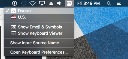
macOS: They keyboard layouts are in System Preferences -> Language & Region -> Keyboard Preferences. Then under Input Sources add a new layout and select Dvorak. Once it’s added there will be an input selector on the right hand side of the Menu Bar by the clock that you can use to switch back and forth.
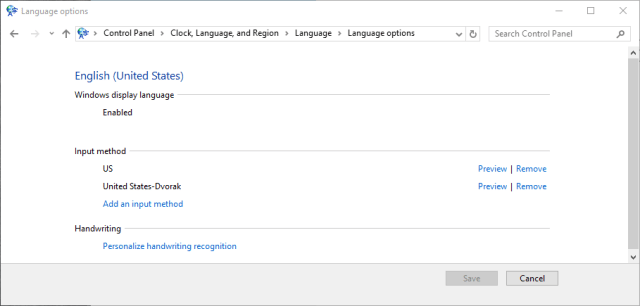
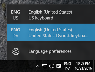
Windows: The layouts can be changed via Control Panel -> Clock, Language, and Region -> Language -> Language Options. Then select “Add an input method” and add Dvorak. Once the new layout is added, there will be an input selection tool by the clock, similar to macOS.
The game Snakes and Ladders is a board game that originated in India a very long time ago. Americans probably know the variant Chutes and Ladders from Milton Bradley, which was first published in 1943. Anybody who has played it enough knows that it can sometimes take a large number of turns to complete, as you keep landing on snakes/chutes that take you backward on the board. This post attempts to quantify exactly how long it can take.
There are variations on the number of squares and placement of the snakes and ladders. For the first part of the discussion I will be using the configuration of the Chutes and Ladders game I own, altough I’ll use the term “snakes” instead of “chutes”, since I’ll be generalizing later to other configurations, and since I’ll be simulating the game using the Python programing language :).
There are 100 spaces, 9 ladders, and 10 snakes. The following figure shows the board with ladders in green and snakes in red.
We can estimate the average number of turns by first considering a board with with no ladders and no snakes. The average spin or roll, having 6 possibilites, is 3.5. Therefore the average number of turns to reach the end would be . Next we consider the contribution of the snakes and ladders, by finding the total number of spaces the ladders move one forward, and the total number of spaces spaces the snakes move one backward. By subtracting the latter from the former we get . We can approximate the impact of the snakes and ladders by assuming the configuration is similar to a board with no snakes and ladders that is longer than the current board by 33 spaces, which accounts for the fact that typically the combination of snakes and ladders move the player backward 33 spaces. Then the average number of turns to reach the end would be . I don’t claim that this is an exact calculation or completely mathematically rigorous, but it should be a decent estimate.
To see how close this estimate is we can simulate the game in code. Then we can have the computer play many games and record the number of turns for a player to win. Then we can look at any statistical properties of the game data we want. The following is a Python program for simulating Snakes and Ladders and creating histograms of the game data using matplotlib and numpy.
# Snakes and Ladders simulation
"""
Copyright (c) 2016 Vernon Miller

Permission is hereby granted, free of charge, to any person obtaining a copy of
this software and associated documentation files (the "Software"), to deal in
the Software without restriction, including without limitation the rights to
use, copy, modify, merge, publish, distribute, sublicense, and/or sell copies
of the Software, and to permit persons to whom the Software is furnished to do
so, subject to the following conditions:

The above copyright notice and this permission notice shall be included in all
copies or substantial portions of the Software.

THE SOFTWARE IS PROVIDED "AS IS", WITHOUT WARRANTY OF ANY KIND, EXPRESS OR
IMPLIED, INCLUDING BUT NOT LIMITED TO THE WARRANTIES OF MERCHANTABILITY,
FITNESS FOR A PARTICULAR PURPOSE AND NONINFRINGEMENT. IN NO EVENT SHALL THE
AUTHORS OR COPYRIGHT HOLDERS BE LIABLE FOR ANY CLAIM, DAMAGES OR OTHER
LIABILITY, WHETHER IN AN ACTION OF CONTRACT, TORT OR OTHERWISE, ARISING FROM,
OUT OF OR IN CONNECTION WITH THE SOFTWARE OR THE USE OR OTHER DEALINGS IN THE
SOFTWARE.
"""

import numpy as np
import matplotlib.pyplot as plt
from random import randint

board = {1:38, 4:14, 9:31, 16:6, 21:42, 28:84, 36:44, 48:26, 49:11, 51:67,
56:53, 62:19, 64:60, 71:91, 80:100, 87:24, 93:73, 95:75, 98:78}

def game(players):
"""Plays one game and return the number of turns taken to win"""
positions = [0 for i in range(players)]
turns = 0
while max(positions) < 100:
for player in range(players):
positions[player] += randint(1, 6) # position after spin/roll
if positions[player] in board:
positions[player] = board[positions[player]]
turns += 1
return turns

N = 1000000   # Number of games to play
nplayers = 1  # Number of players
nbins = 50     # Number of histogram bins
nturns = []   # List to store results
# Play
nturns = []
for i in range(N):
nturns.append(game(nplayers))

nturns = np.array(nturns)
print(np.min(nturns), np.max(nturns), np.mean(nturns))
fig = plt.figure()
plt.title("Players = %d" % nplayers)
plt.xlabel("Turns")
plt.ylabel("Probability")
plt.hist(nturns, bins=nbins, normed=True)
fig.savefig("plot1.png")
plt.hist(nturns, bins=nbins, normed=True, cumulative=True, color="blue")
fig.savefig("plot2.png")
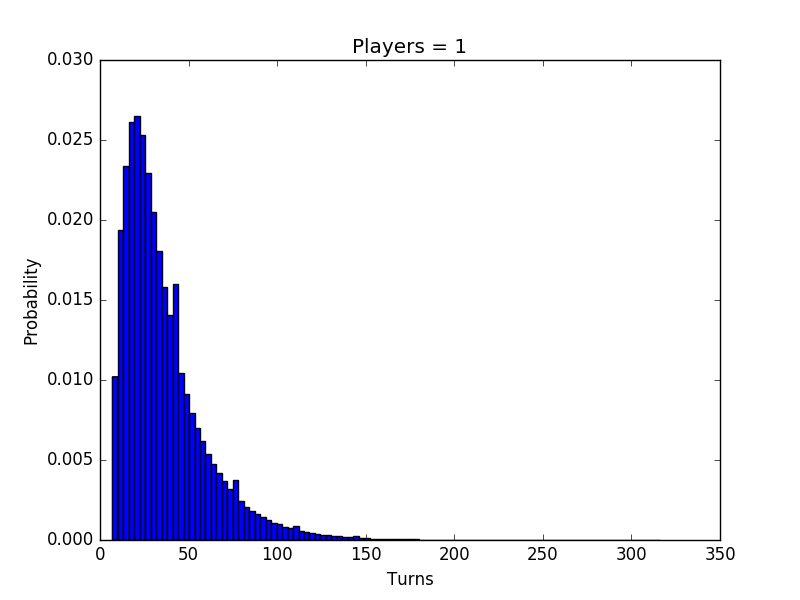
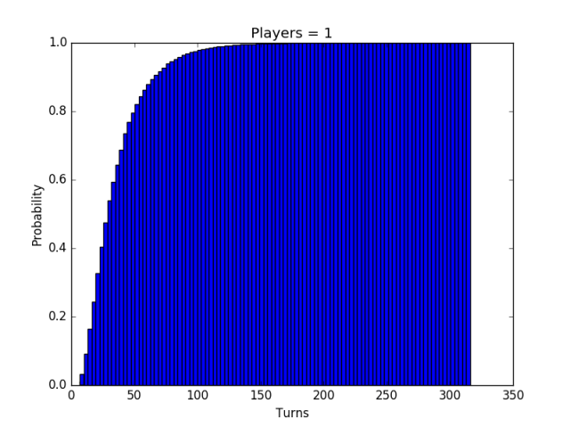
The program produces two histograms that correspond to the probabilty density function and the cumulative density function, respectively. If we play one million single player games we get the following two histograms.
Probability distribution function for Snakes and Ladders
Cumulative distribution function for Snakes and LaddersThe mean number of turns for all one million games was 36.2, which is not too far off the initial estimate of 38. What I really want to point out though is the long tail of the distribution. Some games take a really long time. In the simulation there was one game that took 316 turns! Looking at the cumulative distribution function we can see that it’s not too uncommon to find yourself in a game that lasts 50 turns or more. There is a roughly 20% chance that a game will last at least 50 turns, and about a 5% chance that a game will last at least 80 turns.
How typical is this particular outcome given the configuration of the board? Could we construct some non-trivial configurations that would result in significantly fewer or more average number of turns? Since it’s easy to simulate any configuration we might as well experiment.
First let’s contstrain the configuration to exactly 10 snakes and 9 ladders, just as we had before. Next, we can define an offset as the net spaces moved backwards or fowards by the combination of snakes and ladders. In the previous example this was -33. In python, if we represent the board as a dictionary as in the example above, then calculating the offset is a one liner:
The reason for defining the offset is that I’m curious is there is a simple dependence on the offset and the average number of turns. I assumed there was earlier when I tried to estimate the number of turns, but a simulation can check. Another constraint will be to limit the offset to be greater than -50 and less than 50.
The procedure then is
Generate a random board with 10 snakes and 9 ladders.
Only use boards whose absolute offset is less than 50.
Simulate many games and record the min, max, and mean number of turns.
Print to the stdout the board configuration for simulations that lead to >2X or <0.5x the average number of turns compared to the base configuration so they can be simulated further later on.
Get a cup of coffee or tea while the simulation runs
Plot the offset vs the average number of turns.
Below is the code for this procedure. It can run for quite a while depending on the number of board configuration to try. For 10,000 boards it ran for roughly 1 hour. I’m sure this could be improved by using the multiprocessing capability of python.
# Snakes and Ladders simulation - random sampling of board configurations
"""
Copyright (c) 2016 Vernon Miller

Permission is hereby granted, free of charge, to any person obtaining a copy of
this software and associated documentation files (the "Software"), to deal in
the Software without restriction, including without limitation the rights to
use, copy, modify, merge, publish, distribute, sublicense, and/or sell copies
of the Software, and to permit persons to whom the Software is furnished to do
so, subject to the following conditions:

The above copyright notice and this permission notice shall be included in all
copies or substantial portions of the Software.

THE SOFTWARE IS PROVIDED "AS IS", WITHOUT WARRANTY OF ANY KIND, EXPRESS OR
IMPLIED, INCLUDING BUT NOT LIMITED TO THE WARRANTIES OF MERCHANTABILITY,
FITNESS FOR A PARTICULAR PURPOSE AND NONINFRINGEMENT. IN NO EVENT SHALL THE
AUTHORS OR COPYRIGHT HOLDERS BE LIABLE FOR ANY CLAIM, DAMAGES OR OTHER
LIABILITY, WHETHER IN AN ACTION OF CONTRACT, TORT OR OTHERWISE, ARISING FROM,
OUT OF OR IN CONNECTION WITH THE SOFTWARE OR THE USE OR OTHER DEALINGS IN THE
SOFTWARE.
"""

import numpy as np
import matplotlib.pyplot as plt
from random import randint

def get_board(snakes, ladders):
board = {}
choices = range(1,101)
for s in range(snakes):
a = choices.pop(randint(0, len(choices) - 1))
b = choices.pop(randint(0, len(choices) - 1))
if b > a:
board[b] = a
else:
board[a] = b
for l in range(ladders):
a = choices.pop(randint(0, len(choices) - 1))
b = choices.pop(randint(0, len(choices) - 1))
if b > a:
board[a] = b
else:
board[b] = a
return board

def game(board):
"""Plays one game and return the number of turns taken to win"""
position = 0
turns = 0
while position < 100:         position += randint(1, 6) # position after spin/roll         if position in board:             position = board[position]         turns += 1         if turns > 100000:  # give up to account for impossible to win boards
return 0
return turns

N = 10000    # Number of games to play per iteration
I = 10000    # Number of iterations
# Play
simdata = {}  # map offset -> [[min, max, mean], [min,max,mean],...]
for i in range(I):
acceptable_board = False
while acceptable_board is False:
b = get_board(10, 9)
offset = sum(map(lambda x:x[1]-x[0], b.items()))
if abs(offset) <= 50:             acceptable_board = True     nturns = []     for j in range(N):         nturns.append(game(b))     nturns = np.array(nturns)     mean = np.mean(nturns)     if offset in simdata:         simdata[offset].append([np.min(nturns), np.max(nturns), mean])     else:         simdata[offset] = [[np.min(nturns), np.max(nturns), mean]]     if mean > 100 or mean < 15:
print i, offset, np.min(nturns), np.max(nturns), mean, b
# Analyze and plot the data
x = []
y = []
points = []
for key, value in simdata.iteritems():
mins, maxs, means = zip(*value)
avg_mean = sum(means)/float(len(means))
points.append([key, avg_mean])
points.sort()
x, y = zip(*points)
# find a trendline
line = np.poly1d(np.polyfit(x, y, 1))
fig = plt.figure()
plt.xlabel("Offset")
plt.ylabel("Average Turns")
plt.plot(x, y, "o")
plt.plot(x, line(x), color="black")
print line
plt.show()
There are some differences between this and the first program, besides the fact that it generates random board configurations according to a range of offsets. The simulation is restricted to a single player, and there is now a maximum number of attempted turns on a given game before giving up. This is because for random placement of snakes and ladders there are some configurations that are unwinnable and would therefore run forever in a simulation. For example if squares 94 through 99 are each the start of a slide, and there is no ladder that ends directly on 100, then the game is unwinnable. I chose a maximum number of turns of 100,000, based on running many simulations and never seeing anything close to that as a valid maximum.
One question that comes to mind is how many different board configurations are there with 10 snakes and 9 ladders? I assert that the answer is the same as the number of combinations of selecting 38 items from 100 choices, or
To prove that this is the correct number I can show that any sequence of 38 randomly selected squares from the board can be used to construct exactly 10 snakes and 9 ladders. Let the list of randomly selected squares be written as . Now let them be broken up into 19 pairs . Next sort each pair, resulting in a new list , where and . Finally we will define two operators. A right arrow when placed between squares represents a ladder connecting two squares. A left arrow when placed between squares represents a snake connecting two squares. Place a between the squares of the first 10 pairs, and place a between the squares of the last 9 pairs. There are then 10 snakes and 9 ladders. Since the inital list of squares was arbitrary the value for the number of combinations holds.
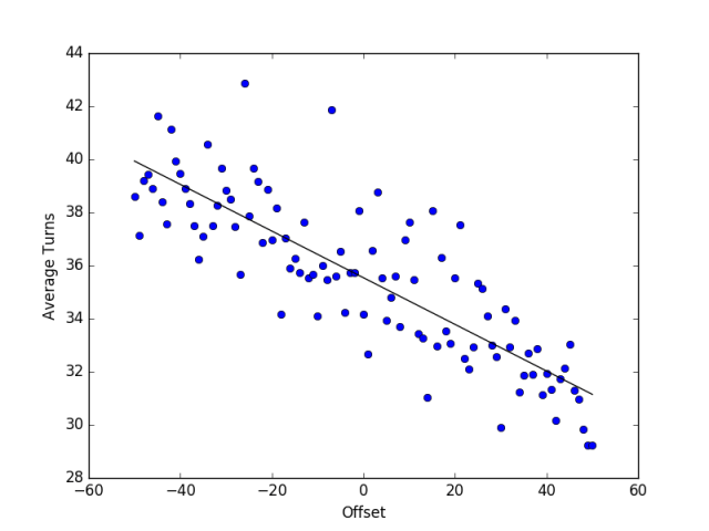
I don’t have enough time to evaluate all 5.6 octillion configurations, so I’ll have to settle for random sampling. The chart below shows the average number of turns (for 10,000 games) for 10,000 random board configurations with varying offsets from -50 to 50.
Random sampling of board configurationsYou can see that at any given offset there is a dense cluster of averages and some outliers. If we could get an average of the averages (actually an average of the means) for each offset then perhaps we can find a linear relationship. The chart below shows the averaged data with a fitted line.
There is a linear relationship in the average behavior over a range of random board configurations for each offsetThe equation for the line, as determined by numpy using a least squares fit, is
Or, with the help of WolframAlpha, we can make the coefficient more memorable and gratuitously complex.
Where is the average number of turns and is the offset.
Let’s take a look at the equation and ask if it makes sense. At first glance by putting in zero for the offset we get 35.54 for the average, and that may seem at odds with the earlier estimate of 28.6 for a board with no snakes and no ladders. However it does make sense because having a zero offset is not the same as having no snakes and ladders, because in all these simulations there were 10 snakes and only 9 ladders. That means that you are more likely to land on a snake than a ladder, and therefore more likely to increase the number of turns to complete the game, even with an offset equal to zero.
If we plug in the offset of -33 from the original configuration into the equation we get 38.5 as the average number of turns. This is pretty close to our initial estimate of 38. There are two things to keep in mind however. We only sampled 10,000 board configurations out of the possible octillion+ possibilities, so with more sampling the fitted line could become more accurate. Also, there are significant outliers, especially those having an average much higher than what would be predicted.
An example of one of the outliers is the board shown below.
Outlier board configuration having a mean of 323 turns to complete a game.This configuration had a mean of 323 turns to complete a game with an offset of -32, which is 8.4x greater than the average for other boards having an offset of -32. In fact one of the simulated games required 2951 turns! It clear that having snakes 6 squares of the top row is the reason.
An outlier on the low side is shown below.
Outlier board configuration having a mean of 15 turns to complete a game.In this case the mean number of turns to complete a game was 15, and the board had an offset of 50. The average number of turns for other boards having an offset of 50 was 31.
Summary
Snakes and ladders has a long tailed distribution for the number of turns required to complete a game, as anybody who has played more than 4 or 5 games has probably experienced.
Calculating an offset based on the particular snakes and ladders provides a decent way finding an average number of turns to complete a game, according to the equation , but there are outliers that deviate significantly.
Python, matplotlib, and numpy are great tools that make simulating games like this very straightforward.
Copyright (c) 2016 Vernon Miller. All Rights Reserved.
As I was falling asleep one night I began to think about regular polygons inscribed in the unit circle. I imagined adding more and more sides to the polygon and watching as the area of the polygon approached the area of the circle. I wondered how to calculate the ratio of the area of the polygon to the circle, and what the curve would look like if I were to plot the values for increasing numbers of sides. I wondered about similar plots for polygons circumscribing the unit circle. I understood that for large numbers of sides the ratio of the areas between the polygon and the circle would approach one, and likewise the ratio of the areas between the inscribed and circumscribed polygons would approach one, albeit more slowly as the circumscribed polygon will always be larger than the unit circle. Would the approach to one be symmetric for the case of the inscribed versus the circumscribed polygon?
Inscribed Polygons
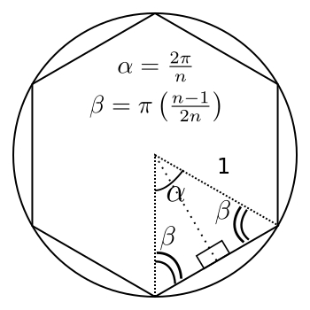
I realized calculating the area of a regular polygon with sides inscribed in the unit circle should be fairly straightforward since any regular polygon can be divided into isosceles triangles sharing a common vertex at the center of the polygon. In this case the equal sides of the triangle have a length of one. Also all of the angles are known, since the interior angle must be .
A regular hexagon inscribed in the unit circle
The triangle can be divided into two right triangles whose non-right angles are and , and each hypotenuse has a length of one. The area of each right triangle is shown to be
In total there are of these triangles per polygon, so the total area of the inscribed polygon, , is therefore
Circumscribed Polygons
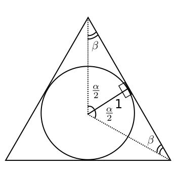
The same procedure as before for calculating area applies to a regular polygon circumscribing the unit circle.
The unit circle inscribed in an equilateral triangle
Finding the area of the right triangle is trivial in this case as the base is just the radius of the unit circle and the height is the tangent of . Therefore the area of each right triangle is . Since there are such triangles the total area of the polgon is
Ratio of Areas
I’m interested in the ratio of the area of the polygon to that of the unit circle and seeing how the ratio changes with various values of . Dividing the equations for the inscribed area and the circumscribed area by the area of the unit circle, , and treating them as functions of , we get
I’m also interested in the ratio of the area of the inscribed polygon to the circumscribed polygon, as this will approach 1 for large just as the previous two equations.
The following figure shows a plot of each function for values from 3 to 30.
The ratio of areas between regular polygons and the unit circle
It’s clear from the plot that and are not symmetric about 1 and that the ratio of the areas of the polygons converges more slowly than the other two functions. However it’s not intuitively clear to me from the ratio equations that the plots should have the shape that they do.
In an attempt to get a simpler explanation of the shape of the curves the ratio functions can be expanded into the first few terms of their respective Taylor series.
The ratio between and is a little bit trickier but we can still eliminate higher order terms for an approximation.
For clarity let .
Finally we arrive at a set of approximate ratio equations that clearly show the trends in the plot.
They show that and are not symmetric around 1 and that has the shallowest approach toward the asymptote.
Copyright (c) 2016 Vernon Miller. All Rights Reserved.


 . Next we consider the contribution of the snakes and ladders, by finding the total number of spaces the ladders move one forward, and the total number of spaces spaces the snakes move one backward. By subtracting the latter from the former we get
  . We can approximate the impact of the snakes and ladders by assuming the configuration is similar to a board with no snakes and ladders that is longer than the current board by 33 spaces, which accounts for the fact that typically the combination of snakes and ladders move the player backward 33 spaces. Then the average number of turns to reach the end would be
  . I don’t claim that this is an exact calculation or completely mathematically rigorous, but it should be a decent estimate.

 . Now let them be broken up into 19 pairs
  . Next sort each pair, resulting in a new list
  , where
  and
and  . Finally we will define two operators. A right arrow
  when placed between squares
  represents a ladder connecting two squares. A left arrow
  when placed between squares
  represents a snake connecting two squares. Place a


 is the average number of turns and
  is the offset.
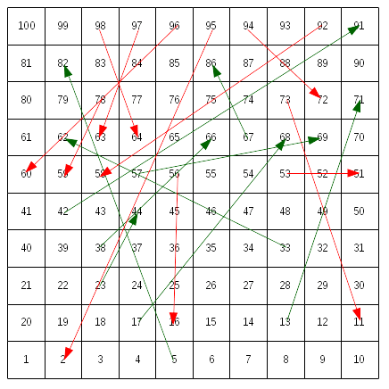

 , but there are outliers that deviate significantly.
 sides inscribed in the unit circle should be fairly straightforward since any regular polygon can be divided into
  .
.
 and
and  , and each hypotenuse has a length of one. The area of each right triangle is shown to be
 of these triangles per polygon, so the total area of the inscribed polygon,
  , is therefore
 . Since there are
 , and treating them as functions of


 and
and  are not symmetric about 1 and that the ratio of the areas of the polygons converges more slowly than the other two functions. However it’s not intuitively clear to me from the ratio equations that the plots should have the shape that they do.
![\begin{aligned} A_I(n) &= \frac{n}{2\pi} \sin\left(\frac{2\pi}{n}\right) \\ &= \frac{n}{2\pi} \left[\frac{2\pi}{n} - \frac{1}{6}{\left(\frac{2\pi}{n}\right)}^3 + \frac{1}{120}{\left(\frac{2\pi}{n}\right)}^5 + \dots\right] \\ &= \frac{n}{2\pi} \left[\frac{2\pi}{n} - \frac{1}{6}{\left(\frac{2\pi}{n}\right)}^3 + \mathcal{O}{\left(\frac{2\pi}{n}\right)}^5\right] \\ &\approx 1 - \frac{2\pi^2}{3n^2} \end{aligned}](https://s0.wp.com/latex.php?latex=%5Cbegin%7Baligned%7D+A_I%28n%29+%26%3D+%5Cfrac%7Bn%7D%7B2%5Cpi%7D+%5Csin%5Cleft%28%5Cfrac%7B2%5Cpi%7D%7Bn%7D%5Cright%29+%5C%5C+%26%3D+%5Cfrac%7Bn%7D%7B2%5Cpi%7D+%5Cleft%5B%5Cfrac%7B2%5Cpi%7D%7Bn%7D+-+%5Cfrac%7B1%7D%7B6%7D%7B%5Cleft%28%5Cfrac%7B2%5Cpi%7D%7Bn%7D%5Cright%29%7D%5E3+%2B+%5Cfrac%7B1%7D%7B120%7D%7B%5Cleft%28%5Cfrac%7B2%5Cpi%7D%7Bn%7D%5Cright%29%7D%5E5+%2B+%5Cdots%5Cright%5D+%5C%5C+%26%3D+%5Cfrac%7Bn%7D%7B2%5Cpi%7D+%5Cleft%5B%5Cfrac%7B2%5Cpi%7D%7Bn%7D+-+%5Cfrac%7B1%7D%7B6%7D%7B%5Cleft%28%5Cfrac%7B2%5Cpi%7D%7Bn%7D%5Cright%29%7D%5E3+%2B+%5Cmathcal%7BO%7D%7B%5Cleft%28%5Cfrac%7B2%5Cpi%7D%7Bn%7D%5Cright%29%7D%5E5%5Cright%5D+%5C%5C+%26%5Capprox+1+-+%5Cfrac%7B2%5Cpi%5E2%7D%7B3n%5E2%7D+%5Cend%7Baligned%7D+&bg=ffffff&fg=111111&s=0&c=20201002)
![\begin{aligned} A_C(n) &= \frac{n}{\pi} \sin\left(\frac{2\pi}{n}\right) \\ &= \frac{n}{\pi} \left[\frac{\pi}{n} - \frac{1}{3}{\left(\frac{\pi}{n}\right)}^3 + \frac{2}{15}{\left(\frac{\pi}{n}\right)}^5 + \dots\right] \\ &= \frac{n}{\pi} \left[\frac{\pi}{n} - \frac{1}{3}{\left(\frac{\pi}{n}\right)}^3 + \mathcal{O}{\left(\frac{\pi}{n}\right)}^5\right] \\ &\approx 1 + \frac{\pi^2}{3n^2} \end{aligned}](https://s0.wp.com/latex.php?latex=%5Cbegin%7Baligned%7D+A_C%28n%29+%26%3D+%5Cfrac%7Bn%7D%7B%5Cpi%7D+%5Csin%5Cleft%28%5Cfrac%7B2%5Cpi%7D%7Bn%7D%5Cright%29+%5C%5C+%26%3D+%5Cfrac%7Bn%7D%7B%5Cpi%7D+%5Cleft%5B%5Cfrac%7B%5Cpi%7D%7Bn%7D+-+%5Cfrac%7B1%7D%7B3%7D%7B%5Cleft%28%5Cfrac%7B%5Cpi%7D%7Bn%7D%5Cright%29%7D%5E3+%2B+%5Cfrac%7B2%7D%7B15%7D%7B%5Cleft%28%5Cfrac%7B%5Cpi%7D%7Bn%7D%5Cright%29%7D%5E5+%2B+%5Cdots%5Cright%5D+%5C%5C+%26%3D+%5Cfrac%7Bn%7D%7B%5Cpi%7D+%5Cleft%5B%5Cfrac%7B%5Cpi%7D%7Bn%7D+-+%5Cfrac%7B1%7D%7B3%7D%7B%5Cleft%28%5Cfrac%7B%5Cpi%7D%7Bn%7D%5Cright%29%7D%5E3+%2B+%5Cmathcal%7BO%7D%7B%5Cleft%28%5Cfrac%7B%5Cpi%7D%7Bn%7D%5Cright%29%7D%5E5%5Cright%5D+%5C%5C+%26%5Capprox+1+%2B+%5Cfrac%7B%5Cpi%5E2%7D%7B3n%5E2%7D+%5Cend%7Baligned%7D&bg=ffffff&fg=111111&s=0&c=20201002)

 .
.

 has the shallowest approach toward the asymptote.